Causal Inference & Analytics Engineering

Complete

F1 Regulation Impact Analyzer

Did Formula 1’s 2022 regulations actually make the competition closer?

Role: Sole analyst & developer
Timeline: Jan–May 2026
Category: Causal Inference & Analytics Engineering
Stakeholder: Personal project

Estimated regulation effect: +0.068Estimated regulation effectDifference-in-differences coefficient, borderline significant at p = 0.050 (HC3 robust SEs).
Lower forecast error vs baseline: 42%Lower forecast error vs baseline2024 walk-forward validation: Ridge MSE 0.0484 vs seasonal-naive 0.0830.
Seasons modelled: 2019–2026Seasons modelledPanel of 8–9 constructors; 2026 is forecast forward from partial-season data.

Snowflake
dbt
Power BI
Python
statsmodels
scikit-learn

In 30 seconds

I built a Snowflake + dbt analytics warehouse and a causal-inference framework to separate the effect of the 2022 rule change from existing team-performance trends, then forecast the 2026 regulation reset with a walk-forward model.

Estimated regulation effect: +0.068Estimated regulation effect
Lower forecast error vs baseline: 42%Lower forecast error vs baseline
Seasons modelled: 2019–2026Seasons modelled

Context

The 2022 Formula 1 regulation overhaul was designed to reduce the dominance of top teams and make the racing closer. That makes it a clean natural experiment: a known intervention, at a known time, applied to some competitors more than others.

The question is the one an analyst faces whenever a policy or market shock lands — did it actually change outcomes, or would the trend have happened anyway? Answering it requires separating the treatment effect from pre-existing trajectories, then forecasting how the system adapts to the next shock (the 2026 reset).

This is a personal project, but the framework — difference-in-differences plus walk-forward forecasting — is exactly what analysts use for pricing changes, competitor entry, and regulation in industry.

Data

Source: FastF1 (timing/results) and the Jolpica/Ergast API (constructor standings)
Time period: 2019–2026 (2026 is partial, forecast forward)
Records: Team-race panel: 1,024 rows (Layer 1, 8 teams, 2019–2024); 1,376 rows (Layer 2, 9 teams, 2019–2026)
Granularity: One row per team per race weekend

Data quality & handling

Outcome variable relative_perf = points per race ÷ race maximum, giving a stable 0–1 scale that controls for varying points available.
McLaren was excluded from the Layer 1 control group: a corporate restructuring in the pre-period confounds their trajectory. They return in Layer 2.
2025 was excluded from Layer 1 — teams were redirecting development to 2026, making that season unrepresentative of the 2022 equilibrium.
The 2020 COVID-compressed season is flagged as an anomaly and retained with a caveat.
All rolling forecast features use closed="left" so a row never sees its own value — preventing data leakage.

Data dictionary

Table	Description	Size
relative_perf	Points per race normalized by race maximum (0–1).	outcome
treated / post	Top-team flag and post-2022 flag; their interaction is the DiD term.	design
rolling_mean	Recent form (leakage-free rolling mean).	feature
yoy_change / season_std	Development trajectory and within-season consistency.	feature

Analytical approach

The warehouse follows a clean lineage: raw parquet → Snowflake RAW → dbt staging (typed views) → dbt marts (tables) that Power BI reads. Three marts back three dashboard views.

Ingest FastF1 + Jolpica
Build team-race panel (Python)
Parallel-trends & placebo checks
Difference-in-differences (statsmodels)
Walk-forward Ridge forecast
Load to Snowflake
Transform in dbt (staging → marts)
Power BI reporting

The report

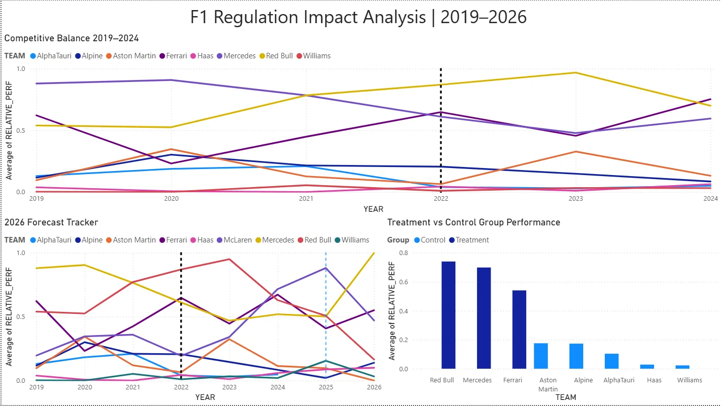
Power BI dashboard showing competitive balance, treatment vs control, and the 2026 forecast tracker. — The three-view Power BI dashboard connected live to Snowflake mart tables.

Findings

The 2022 rules produced a small, borderline-significant convergence effect.

The difference-in-differences estimate is +0.068 at p = 0.050 — directionally consistent with top teams losing a modest relative edge, but not a strong causal claim.

Why it matters. It quantifies a policy shock honestly: the regulation nudged competitive balance rather than overhauling it, matching Red Bull’s rapid return to dominance by 2023.

Caveat. p = 0.050 is marginal; constructor budgets (a known confounder) are not publicly available.

Average performance: treatment vs control

Average performance: treatment vs control
Team	Average relative performance
Red Bull	0.745
Mercedes	0.700
Ferrari	0.545
Aston Martin	0.175
Alpine	0.170
AlphaTauri	0.105
Haas	0.030
Williams	0.025

Recreated as native SVG from the project’s output (Power BI dashboard, did_results.txt).

A Ridge model beats a naïve baseline by 42% in 2024.

Walk-forward validation shows the model learning regulation-response patterns as post-2022 data accumulates, with 2024 MSE of 0.0484 versus 0.0830 for the seasonal-naive baseline.

Why it matters. It demonstrates an adaptive forecast that improves as actuals arrive — the same pattern used in demand and churn forecasting.

Caveat. The 2022 reset year is a tie: no model can predict a regulation change before it happens.

Walk-forward MSE: Ridge vs seasonal-naive

Walk-forward MSE: Ridge vs seasonal-naive
Validation year	Mean squared error
Ridge 2022	0.051
Ridge 2023	0.051
Ridge 2024	0.048
Ridge 2025	0.061
Seasonal naive 2022	0.051
Seasonal naive 2023	0.055
Seasonal naive 2024	0.083
Seasonal naive 2025	0.064

Recreated as native SVG from the project’s output (forecast_results.csv, seasonal_naive_results.csv).

Parallel-trends checks pass for 2019 but fail for 2020.

The 2019 placebo passed; the 2020 placebo failed and is attributed to the COVID-compressed calendar, an acknowledged anomaly retained with a caveat.

Why it matters. Validating the DiD assumption before trusting the estimate is what separates a defensible causal claim from a spurious one.

Pre-regulation parallel-trends check (2019–2021)

Pre-regulation parallel-trends check (2019–2021)
Year	Relative performance
Treatment 2019	0.680
Treatment 2020	0.555
Treatment 2021	0.672
Control 2019	0.078
Control 2020	0.168
Control 2021	0.122

Recreated as native SVG from the project’s output (pre_reg_parallel_trends.png).

Recommendations

Apply the same DiD-plus-walk-forward framework to business policy shocks.

What the analysis suggests

Evidence: The design cleanly separates a treatment effect from pre-existing trends — the analyst’s task in pricing changes, competitor entry, and regulation.
Expected benefit: A reusable template for measuring causal impact and tracking forecasts against live actuals.

Validation

Parallel-trends & placebo tests
Trends were checked visually and with placebo treatment years before running DiD. The 2019 placebo passed; the 2020 placebo failed and is disclosed as a COVID anomaly.
Robust inference
OLS with team fixed effects (absorbing time-invariant team quality) and HC3 heteroskedasticity-consistent standard errors. The DiD term is +0.068 at p = 0.050.
Walk-forward validation
The forecast is validated year by year against a seasonal-naive baseline, beating it in 2023–2025 and tying at the 2022 reset (which no model can predict).
Leakage prevention
Every rolling feature excludes the current row (closed="left"), so no future information enters training.

Limitations

The DiD coefficient at p = 0.050 is borderline; the effect is real in direction but modest in magnitude.
The 2020 placebo failure (COVID season) violates parallel trends for that year.
Constructor budgets are not public — an unmodelled confounder for team performance.
The 2026 validation set is small because the season is still early.

My contribution

Built the FastF1 + Jolpica data pipeline and the Snowflake + dbt warehouse (staging → marts).
Specified and ran the DiD model with team fixed effects and HC3 robust standard errors.
Engineered leakage-free walk-forward features and the Ridge forecasting model.
Designed the three-view Power BI reporting layer connected live to Snowflake.

Technical appendix

Difference-in-differences output (key terms)

OLS on relative_perf with team fixed effects and HC3 robust standard errors (N = 1,024, R² = 0.601). The post × treated interaction is the causal estimate.

                              coef    std err      z     P>|z|
post                       -0.0344     0.013    -2.596    0.009
post:treated                0.0682     0.035     1.963    0.050
C(team)[T.Red Bull]         0.6006     0.039    15.473    0.000
C(team)[T.Mercedes]         0.5592     0.038    14.606    0.000
C(team)[T.Ferrari]          0.4010     0.037    10.758    0.000
Covariance Type: HC3   |   R-squared: 0.601   |   N: 1024

Warehouse & dashboard

Snowflake (F1_WH X-Small, F1_DB) holds RAW, staging and mart schemas built by dbt. Three marts — competitive balance, DiD effects, and the 2026 forecast tracker — feed a three-view Power BI report connected live to Snowflake.

Forecasting model

Ridge regression was chosen over tree models given the small panel (1,024 rows): regularization helps and coefficients stay interpretable. Features capture recent form, year-over-year trajectory, and within-season consistency, plus treatment/regulation-era flags.