Spatial & Operational Analytics

Complete

Halifax Transit Service Equity Analysis

Where is Halifax’s transit network leaving riders underserved?

Role: Sole analyst & developer
Timeline: Dec 2025
Category: Spatial & Operational Analytics
Stakeholder: Personal project (framed for a municipal transit-planning stakeholder)

Transit records analysed: 663,788Transit records analysedGTFS static feed across 11 normalized tables (481,610 stop-time entries).
Stops served by a single route: 41%Stops served by a single routeA connectivity gap: 973 stops (of 2,380) depend on one route only.
Query time, down from 4s+: <1sQuery time, down from 4s+Stop-connectivity view optimized via B-tree and GIST spatial indexes.

SQL
PostgreSQL
PostGIS
Python
Streamlit

In 30 seconds

I transformed 663,788 public-transit records into a normalized PostgreSQL + PostGIS spatial database and an interactive dashboard, surfacing gaps in route access, stop connectivity, and service concentration across Halifax.

Transit records analysed: 663,788Transit records analysed
Stops served by a single route: 41%Stops served by a single route
Query time, down from 4s+: <1sQuery time, down from 4s+

Context

Halifax publishes its transit schedule as an open GTFS feed, but the raw feed is a set of flat files — useful for trip planning, not for asking whether the network serves riders evenly. There was no queryable, spatial view of where coverage thins out.

This project treats the feed as an analytics problem: could a normalized spatial database and dashboard reveal the parts of the network where access, connectivity, and frequency fall short — the kind of evidence a municipal transit planner would need to target improvements?

It is a personal project. The stakeholder is framed, not real, so the recommendations are written as what the analysis suggests rather than a mandate.

Data

Source: Halifax Transit GTFS static feed (public open data)
Time period: Schedule snapshot, December 2025
Records: 663,788 records across 11 normalized tables
Granularity: 2,380 stops · 80 routes · 13,666 trips · 481,610 stop-time entries

Data quality & handling

Foreign-key integrity checks filtered 10 invalid trips (0.07%) and 65 invalid calendar dates before load.
ID fields arrived inconsistently typed (VARCHAR in schema, INTEGER from CSV); all IDs were normalized to strings so joins resolved.
Date fields were converted from YYYYMMDD integers to PostgreSQL DATE types.
The feed is a scheduled snapshot — it records planned service, not real-time vehicle positions or ridership.

Data dictionary

Table	Description	Size
stops	Stop locations; PostGIS geometry auto-populated from lat/lon.	2,380 rows
routes	Route identifiers and metadata.	80 rows
trips	Scheduled trips linking routes to service patterns.	13,666 rows
stop_times	Arrival/departure per stop per trip — the analytical grain.	481,610 rows

Analytical approach

PostGIS geometry columns are populated automatically from stop coordinates via triggers, and GIST spatial indexes make distance queries fast enough for interactive use.

Ingest the GTFS static feed
Validate & normalize (FK checks, ID/date types)
Load to PostgreSQL + PostGIS
Build SQL analytical views
Spatial analysis (PostGIS)
Temporal analysis
Streamlit dashboard

The report

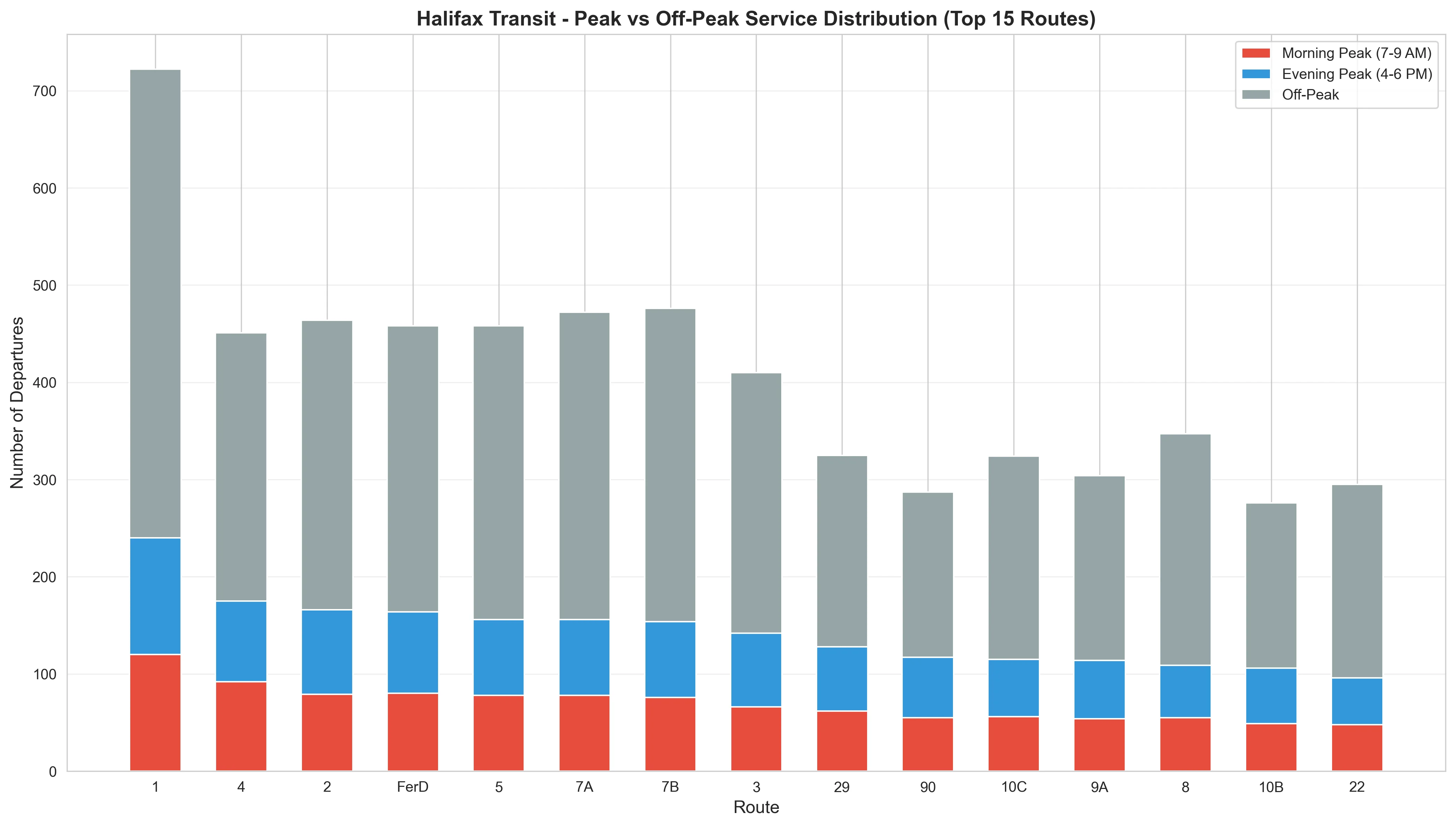
Stacked bar chart of the top 15 Halifax Transit routes, splitting each route’s departures into morning peak (7–9 AM), evening peak (4–6 PM) and off-peak service. — Peak versus off-peak service distribution across the fifteen busiest routes — Route 1 carries roughly 50% more departures than any other.

Findings

Service is highly concentrated on a few core routes.

Route 1 (Spring Garden) runs about 180 trips per service pattern — far above the next-busiest routes — and the Barrington St hub serves 27 routes.

Why it matters. A handful of trunk routes carry the network. Their reliability disproportionately shapes the rider experience city-wide.

Route frequency — top 10 routes

Route frequency — top 10 routes
Route	Avg trips per service pattern
1	180
7B	119
7A	118
2	116
5	114
4	112
3	102
FerD	91
8	86
9A	76

Recreated as native SVG from the project’s output (route_frequency.png).

41% of stops are served by a single route.

Of 2,380 stops, 973 are served by only one route, and average connectivity is 2.17 routes per stop. Only 152 stops (6%) act as hubs with five or more routes.

Why it matters. Single-route stops leave riders with no alternative when a route is delayed or cut — a structural fragility in the network.

Caveat. Based on the scheduled GTFS feed, not observed ridership; it measures service supply, not demand.

Stop connectivity distribution

Stop connectivity distribution
Routes serving a stop	Number of stops
1	973
2	875
3	220
4	150
5	52
6	15
7	30
8	18
9	14
10+	33

Recreated as native SVG from the project’s output (stop_distribution.png).

Service peaks sharply at 17:00 with 33,635 departures.

Demand-shaped scheduling produces a clear morning (7–9 AM) and evening (4–6 PM) commuter pattern, with the evening rush the busiest window.

Why it matters. Off-peak and midday coverage is comparatively thin, which shapes access for non-commuter trips.

Departures by hour of day

Departures by hour of day
Hour of day	Departures
5	4,100
6	24,200
7	31,200
8	30,800
9	27,000
10	24,400
11	24,100
12	24,300
13	24,300
14	25,100
15	28,400
16	32,500
17	33,635
18	31,900
19	23,200
20	21,400
21	20,800
22	18,400
23	15,200

Recreated as native SVG from the project’s output (hourly_service.png).

Sunday service runs 47% below weekday levels.

Weekday scheduled trips (4,195) fall to 2,217 on Sundays — a 47% reduction confirmed directly in the schedule data.

Why it matters. Weekend service reductions disproportionately affect riders who depend on transit for non-standard work hours.

Caveat. Reflects scheduled service; special-event or seasonal adjustments are not modelled.

Scheduled trips by day type

Scheduled trips by day type
Day type	Scheduled trips
Weekday	4,195
Saturday	2,765
Sunday	2,217

Recreated as native SVG from the project’s output (weekday_weekend.png).

Recommendations

Prioritize connectivity upgrades at high-isolation single-route stops.

What the analysis suggests

Evidence: 973 single-route stops concentrated away from the downtown hub cluster.
Expected benefit: Improves network resilience and rider access with targeted, low-cost route overlaps.

Validation

Data-quality tests
A validation layer in the ETL pipeline queried referenced tables to build valid ID sets and filtered the dataframe before insertion, removing invalid trips and calendar dates.
Manual spot checks
Results were checked against known ground truth — Route 1 (Spring Garden) as the highest-frequency route and Barrington St as the busiest transfer hub (27 routes).
Query-plan verification
EXPLAIN ANALYZE identified sequential scans and a disk-based merge sort on the 481,610-row connectivity view; adding B-tree and GIST indexes cut execution from 4s+ to under 1s.
Reproducibility
Schema, analytical views, and the ETL pipeline are scripted, so the database can be rebuilt from the raw feed end to end.

Limitations

Uses the scheduled GTFS static feed — it describes planned service, not actual vehicle performance or ridership.
“Equity” here means spatial service access (coverage, connectivity, isolation); demographic equity was not analysed as no demographic data was joined.
A single schedule snapshot; seasonal and special-service variations are out of scope.
Isolation is measured as straight-line distance to the nearest neighbouring stop, which is not the same as walking distance over the street network.

My contribution

Designed the PostgreSQL + PostGIS schema and ETL pipeline end to end.
Authored the analytical SQL views and the Streamlit dashboard.
Diagnosed and fixed the query-performance bottleneck (4s+ → <1s).

Technical appendix

Query performance optimization

The stop-connectivity view joined stop_times (481,610 rows) and initially took 4+ seconds, using an external merge sort spilling ~39MB to disk. Adding B-tree indexes on the foreign keys (trip_id, stop_id, route_id, service_id) and GIST indexes on the geometry columns brought it under one second, and Streamlit result caching kept the dashboard responsive.

Analytical SQL views

Four views encapsulate the analysis: route_summary (trips, patterns, unique stops per route), route_efficiency (average trips per service pattern), stop_connectivity (routes per stop, hub identification), and busiest_stops (ranked by daily service volume).

Data model

11 normalized tables follow the GTFS specification with foreign-key constraints. PostGIS geometry columns are auto-populated from lat/lon via triggers, and spatial indexes support ST_Distance proximity queries.